
TreeBoosting-03: Why Does XGBoost Win Every Machine Learning Competition?
Introduction
-
In this part of the Tree Boosting series, we have already talked about the basics of decision trees which are used as base leaners of tree boosting algorithms. We also discussed several approaches of building ensembling models from decision trees such as bagging, random forests and boosting.
-
In this post, we will dive deep into tree boosting methods and then answer the question “Why Does XGBoost Win “Every” Machine Learning Competition?”. The content of this post was extracted from a one-hundred-page paper named Tree Boosting With XGBoost
Supervised Learning
Supervised learning is a part of Machine Learning, which is concerned with modelling the relationship between a response variable $Y$ and a set of predictor variables $X$.
Predictive Modelling
There are two kinds of modelling - explanatory and predictive. In explanatory modelling, we are interested in understanding the causal relationship between $X$ and $Y$, while predictive modelling is concerned with predicting $Y$ by using $X$ as predictors. From now on, we will concern ourself with predictive modelling.
The Loss Function
In the statistical view, predictive modelling can be viewed as a problem of function estimation. The prediction accuracy of the function is measured using a loss function, which measures the discrepancy between a prediction and the true outcome.
\[L(y, f(x))\]In theory we can use any loss function that reflect discrepancy between the observations and the predictions. In practice however, there are a few popular loss functions which tend to be used for a wide variety of problems. Many of the loss functions used in practice are likelihood-based, i.e. negative log-likelihoods.
Likelihood-based Loss Functions
For regression, we assume a conditional Gaussian distribution
\[[Y | X] \sim Normal(\mu(X), \sigma^2).\]The loss function based on this likelihood is
\[L(y, \mu(x)) = \frac{1}{2} log 2\pi\sigma^2 + \frac{1}{2\sigma^2} (y − \mu(x))^2.\]Maximum likelihood estimation with a Gaussian error assumption is however equivalent to least-squares regression as the loss function is equivalent to the squared error loss
\[L(y, f(x)) = (y − f(x))^2.\]For binary classification, the Bernoulli distribution is useful. Letting $ \mathcal{Y} = \{ 0, 1 \} $, we can assume
\[[Y |X] \sim Bernoulli(p(X)).\]The loss function based on this likelihood is
\[L(y, p(x)) = −y log(p(x)) − (1 − y) log(1 − p(x))\]where
\[p(x) = Prob[Y = 1|X = x].\]The loss function based on the Bernoulli likelihood is also referred to as the log-loss, the cross-entropy or the Kullback-Leibler information.
The Risk Function
While the loss function measures the accuracy of a prediction after the outcome is observed. At the time we make the prediction however, the true outcome is still unknown, and the loss incurred is consequently a random variable $L(Y, f(X))$. The true risk of function $f$ is defined as the expected loss
\[R(f) = E[L(Y, f(X))]\]The target function is now defined as
\[f^{*} = \underset{f}{\arg\min} R(f)\]and the goal is to estimate this target function.
Empirical Risk Minimization
Unfortunately, since we may never know the true risk $R(f)$, we need to rely on the empirical risk when inferring our model.
\[\hat{R}(f) = \frac{1}{n} \sum\limits_{i=1}^n L(y_i, f(x_i))\]By the strong law of large numbers we have that
\[\lim_{n\to\infty} \hat{R}(f) = R(f),\]almost surely.
The problem of function estimation is now to estimate the empirical target function
\[\hat{f} = \underset{f\in\mathcal{F}}{\arg\min} \hat{R}(f).\]Empirical risk minimization (ERM) is an induction principle which relies on minimization of the empirical risk. ERM is a criterion to select the optimal function $\hat{f}$ from a set of functions $\mathcal{F}$, so called model class. The choice of $\mathcal{F}$ is of major importance.
The perhaps most popular model class is the class of linear models
\[\mathcal{F} = \{ f : f(x) = \theta_0 + \sum\limits_{j=1}^p \theta_j x_j \} .\]The Learning Algorithm
The model class together with the ERM principle reduces the learning problem to an optimization problem. The computational aspect of the problem is to actually solve the the optimization problem defined by ERM. This is the job of the learning algorithm, which is essentially just an optimization algorithm.
The learning algorithm takes a data set $\mathcal{D}$ as input and outputs a fitted model $\hat{f}$. Most of model classes will have some parameters $\theta$ that the learning algorithm will adjust to fit the data. In this case, model estimation becomes estimating the parameters $\theta$.
\[\hat{f}(x) = f(x;\theta)\]Common learning methods include
- The Constant
- Linear Methods
- Local Regression Methods
- Basis Function Expansions
- Adaptive Basis Function Models
The Optimization Algorithm
Different choices of model classes and loss functions will lead to different optimization problems varying in dificulty and thus requiring different approaches. The simplest problems yield analytic solutions. Most problems do however require numerical methods.
When the objective function is continuous with respect to $\theta$ we get a continuous optimization problem. When this is not the case, we have a discrete optimization problem. The continuous optimization problems are typically easier to solve than discrete optimization problems thus are more desirable when it comes to choose the model class and loss function.
One notable example of a model class which leads to a discrete optimization problem is tree models. Most model classes does however lead to continuous optimization problems. There are numerous methods for continuous optimization problems. Two prominent methods that will be important for tree boosting implementation however, is the method of gradient descent and Newton’s method. Gradient boosting and Newton boosting are approximate nonparametric versions of these optimization algorithms.
Numerical Optimization in Parameter Space
Assume that we are trying to fit a model $f(x) = f(x;\theta)$ parameterized by $\theta$ then the risk of the model can be written as
\[R(\theta) = E[L(Y,f(X;\theta))]\]Given that $R(\theta)$ is differentiable with respect to $\theta$ we can estimate $\theta$ using a numerical optimization algorithm such as gradient descent or Newton’s method.
For both algorithms, at iteration $m$, the estimate of $\theta$ is updated according to
\[\theta^{(m)} = \theta^{(m-1)} + \theta_m\]where $\theta_m$ is the step taken at iteration $m$.
The resulting estimate of $\theta$ after $M$ iterations can be written as a sum
\[\theta \equiv \theta^{(M)} = \sum\limits_{m=0}^M \theta_m,\]where $\theta_0$ is an initial guess and $\theta_1$, …, $\theta_M$ are the successive steps taken by the optimization algorithm.
The difference between two algorithms is in the step $\theta_m$ they take.
Gradient Descent
At each interation, gradient descent takes a step along the direction of steepest descent of the risk given by
\[−g_m = −\nabla_\theta R(\theta)|_{\theta=\theta^{(m−1)}}.\]To surely reduce risk however, the length of the step taken should be not too long. A popular way to determine the step length $\rho_m$ to take in the steepest descent direction is to use line search
\[\rho_m = \underset{\rho}{\arg\min} R(\theta^{(m-1)} - \rho g_m).\]The step taken at iteration $m$ can thus be written
\[\theta_m = −\rho_m g_m.\]Newton’s Method
Unlike gradient descent, Newton’s method determines both the step direction and step length at the same time. Newton’s method can be motivated as a way to approximately solve
\[\nabla_{\theta_m} R(\theta^{(m−1)} + \theta_m) = 0\]By doing a second-order Taylor expansion, we get
\[\nabla_{\theta_m} R(\theta^{(m−1)} + \theta_m) \approx g_m + H_m \theta_m = 0\]where $H_m$ is the Hessian matrix at the current estimate
\[H_m = \nabla_{\theta}^2 R(\theta)|_{\theta=\theta^{(m−1)}}.\]The solution to this is given by
\[\theta_m = −H_m^{−1} g_m.\]From the discussion above, we can see that Newton’s method is a second-order method, while gradient descent is a first-order method.
Boosting
Boosting refers to a class of learning algorithms that fit the data by combining multiple simple models. Each simple model is learnt using a base learner or weak learner which tend to have a limited predictive ability, but when selected carefully using a boosting algorithm, they form a relatively more accurate model. This is the meaning of “boosting”.
AdaBoost is regarded as the first practical boosting algorithm for binary classification. This algorithm fits a weak learner to weighted versions of the data iteratively. At each iteration, the weights are updated such that the misclassified data points recieve higher weights.
The resulting model can be written
\[\hat{f}(x) \equiv \hat{f}^{(M)}(x) = \sum\limits_{m=1}^M \hat{\theta}_m \hat{c}_m(x)\]where $\hat{c}_m(x) \in \{ −1, 1 \} $ are the weak classifiers and hard classifications are given by $\hat{c}_m(x) = sign(\hat{f}(x))$.
In the statistical view of the algorithm, it has been shown that AdaBoost was actually minimizing the exponential loss function
\[L(y,f(x)) = e^{−yf(x)}.\]The early work on boosting focused on binary classification. After that, the view of boosting algorithms as numerical optimization techniques was developed. This led to the development of general boosting algorithms, e.g. gradient boosting, that allowed for optimization of any differentiable loss function. Boosting became applicable to general regression problems and not only classification.
Numerical Optimization in Function Space
Above, we have discussed numerical optimization in parameter space. We will now discuss numerical optimization in function space.
Note that minimizing
\[R(f) = E[L(Y, f(X))]\]is equivalent to minimizing
\[R(f(x)) = E[L(Y, f(x))|X = x]\]At a current estimate $f^{(m−1)}$, the “step” $f_m$ is taken in function space to obtain $f^{(m)}$. Analogously to parameter optimization update we can write the update at iteration $m$ as
\[f^{(m)}(x) = f^{(m−1)}(x) + f_m(x)\]The resulting estimate of $f$ after $M$ iterations can be written as a sum
\[f(x) \equiv f^{(M)}(x) = \sum\limits_{m=0}^M f_m (x),\]where $f_0$ is an initial guess and $f_1$,…, $f_M$ are the successive “steps” taken in function space.
Gradient Descent in Function Space
Similar to the case of gradient descent in parameter space, we have the direction of steepest descent of the risk by taking the negative gradient
\[−g_m(x) = − E \left[ \frac{\partial L(Y,f(x))}{\partial f(x)} | X=x \right]_{f(x)=f^{(m−1)}(x)}\]The step length $\rho_m$ to take in the steepest descent direction can be determined using line search
\[\rho_m = \underset{\rho}{\arg\min} E[L(Y, f^{(m−1)}(X) − \rho g_m(X)].\]The “step” taken at each iteration $m$ is then given by
\[f_m(x) = −\rho_m g_m(x).\]Performing updates iteratively according to this yields the gradient descent algorithm in function space.
Newton’s Method in Function Space
The Newton “step” in function space is given by
\[f_m (x) = − \frac{g_m(x)}{h_m(x)}\]where $h_m(x)$ is the Hessian at the current estimate
\[h_m(x) = E \left[ \frac{\partial^2 L(Y,f(x))}{\partial f(x)^2} | X=x \right]_{f(x)=f^{(m−1)}(x)}.\]Boosting Algorithms
As seen from the previous sections, boosting fits ensemble models of the kind
\[f(x) = \sum\limits_{m=0}^M f_m(x).\]These can be rewritten as adaptive basis function models
\[f(x) = \theta_0 + \sum\limits_{m=1}^M \theta_m \phi_m(x),\]where $f_0(x) = \theta_0$ and $f_m(x) = \theta_m \phi_m(x)$ for $m = 1, …M$.
Most boosting algorithms can be seen to solve
\[\{ \hat{\theta}_m, \hat{\phi}_m \} = \underset{ \{ \theta_m, \phi_m \} }{\arg\min} \sum\limits_{i=1}^n L(y_i, \hat{f}^{(m−1)}(x_i) + \theta_m \phi_m(x_i))\]either exactly or approximately at each iteration. Gradient boosting and Newton boosting can be viewed as general algorithms that solve the equation approximately for any suitable loss function. Also, gradient boosting and Newton boosting can be viewed as empirical versions of the numerical optimization algorithms in function space we developed above.
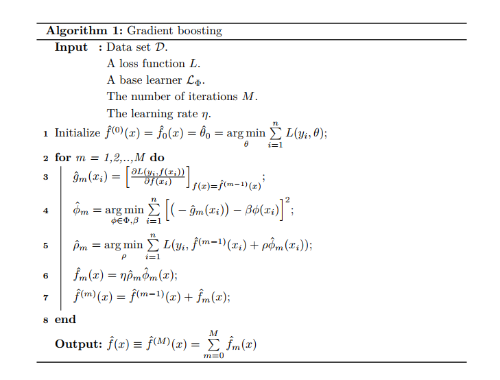
Gradient Boosting
The development of gradient boosting is based on gradient descent in function space that we derived before. Here, the empirical risk will take the place of the true risk.
The empirical version of the negative gradient is given by
\[−\hat{g}_m(x_i) = − \left[ \frac{\partial L(y_i,f(x_i))}{\partial f(x_i)}\right]_{f(x)=f^{(m−1)}(x)}\]Note that this empirical gradient is only defined at the data points $ \{ x_i \}_{i=1}^n $. Thus, to generalize to other points and prevent overfitting, we need to learn an approximate negative gradient using a set of basis functions $\Phi$.
At iteration $m$, the basis function $\phi_m \in \Phi$ is learnt from the data such that it produces output $ \{ \phi_m(x_i) \}_{i=1}^n $ which is most highly correlated with the negative gradient. This is obtained by
\[\hat{\phi}_m = \underset{\phi_m \in \Phi, \beta}{\arg\min} \sum\limits_{i=1}^n \Big[ (− \hat{g}_m(x_i)) − \beta \phi(x_i)\Big]^2\]The basis function $\phi_m$ is learnt using a base learner where the squared error loss is used as a surrogate loss. The step length ρm to take in this step direction can subsequently be determined using line search
\[\hat{\rho}_m = \underset{\rho}{\arg\min} \sum\limits_{i=1}^n L(y_i, \hat{f}^{(m−1)}(x_i) + \rho \hat{\phi}_m(x_i)).\]A regularization technique is also used where the step length at each iteration is multiplied by some factor $0 < \eta \leq 1$. The factor $\eta$ is sometimes referred to as the learning rate as lowering it can slow down learning.
Combining all this, the “step” taken at each iteration $m$ is given by
\[\hat{f}_m(x) = \eta \hat{\rho}_m \hat{\phi}_m(x).\]Doing this iteratively yields the gradient boosting procedure.
Gradient Boosting Algorithm
Newton Boosting
Similar to the case for gradient boosting, we have that the empirical gradient is defined solely at the data points. We thus also need a base learner here to select a basis function from a restricted set of functions. The Newton “step” is found by solving
\[\hat{\phi}_m = \underset{\phi \in \Phi}{\arg\min} \sum\limits_{i=1}^n \frac{1}{2} \hat{h}_m(x_i) \Big[\frac{\hat{g}_m(x_i)}{\hat{h}_m(x_i)} + \phi(x_i) \Big]^2\]where $\hat{g}_m(x_i)$ is the gradient and $\hat{h}_m(x_i)$ is the Hessian matrix.
The “step” taken at each iteration $m$ is given by
\[\hat{f}_m (x) = \eta \hat{\phi}_m(x).\]Repeating this iteratively yields the Newton boosting procedure. Note that the boosting algorithm developed here is the one used by XGBoost.
Newton Boosting Algorithm

Tree Boosting Methods
Using trees as base models for boosting is a very popular choice. In practice, gradient boosting has been particularly successful when applied to tree models, in which case it fits additive tree models. We will refer to this method as MART (Multiple Additive Regression Trees), but it is also known as GBRT (Gradient Boosted Regression Trees) and GBM (Gradient Boosting Machine), which was devised by Friedman in 2001, 2002. More recently, a new tree boosting method has come to stage and quickly gained popularity. It goes by the name XGBoost by Chen and Guestrin in 2016. While both tree boosting methods are conceptually similar, they however differs in multiple ways, i.e. regularization techniques they offer and the boosting algorithm they employ.
Boosted tree models can be viewed as adaptive basis function models.
\[f(x) = \theta_0 + \sum\limits_{m=1}^M f_m (x)\]Boosting tree models results in a sum of multiple trees $f_1$, …, $f_M$. They are therefore also referred to as tree ensembles or additive tree models. While the predictive ability is great increased through boosting, the main drawback of boosted tree models compared to single tree models is that most of the interpretability is lost.


Regularization
Complexity Constraints
There are three ways of controlling the complexity of an additive tree model:
- Constraining the number of trees.
- Restricting the maximum number of terminal nodes of each individual tree.
- Limiting the minimum number of observations falling in any terminal node.
For additive tree models, shallow regression trees are commonly used, i.e. regression trees with few terminal nodes.
Complexity Penalization
One of the core improvements of XGBoost over MART is that it offers the possibility of penalizing the complexity of the trees. The penalty is the sum of the complexity penalties of the individual trees in the additive tree model.
\[\omega(f) = \sum\limits_{m=1}^M \left[ \gamma T_m + \frac{1}{2} \lambda ||w_m||_2^2 + \alpha ||w_m||_1 \right].\]We see that the regularization term includes penalization of the number of terminal nodes of each individual tree through $gamma$, $l_2$ regularization of the leaf weights and $l_1$ regularization on the term weights.
Randomization
Introducing randomness in the learning procedure could improve generalization performance. Two common methods are row subsampling and column subsampling. At each boosting iteration, row subsampling draws a random sample of the data without replacement, which slightly differs from bootstrapping method. Meanwhile, column subsampling means randomly sampling the predictors which is similar to the idea used in Random Forests.
MART includes row subsampling, while XGBoost includes both row and column subsampling. The row and column subsampling fraction $0 < w_r, w_c < 1$ are the two randomization hyperparameters for the boosting procedure in XGBoost.
Learning Algorithms
When fitting additive tree models, MART and XGBoost employ two different tree boosting algorithms which are gradient tree boosting (GTB) and Newton tree boosting (NTB), respectively. For simplicity, we will assume the objective is the empirical risk without any penalization. They are thus learning algorithms for solving the same empirical risk minimization problem.
The optimization problem is simplified by doing forward stagewise additive modeling (FSAM). This simplies the problem by performing a greedy search, adding one tree at a time. At iteration $m$, both these algorithms seek to minimize the FSAM criterion
\[J_m (\phi_m) = \sum\limits_{i=1}^n L(y_i, \hat{f}^{(m−1)}(x_i) + \phi_m (x_i)).\]where the basis functions are trees
\[\phi_m(x) = \sum\limits_{j=1}^T w_{jm} I(x \in R_{jm}).\]While Newton tree boosting is simply Newton boosting with trees as basis functions, gradient tree boosting is a modification of regular gradient boosting to the case where the basis functions are trees. We will in this section show how Newton tree boosting and gradient tree boosting learns the tree structure and leaf weights at each iteration.
Newton Tree Boosting Algorithm
The Newton tree boosting algorithm is simply the Newton boosting shown in Algorithm 2 where the basis functions are tree models. As dicussed above, Newton boosting approximates the FSAM criterion by
\[\tilde{J}_m (\phi_m) = \sum\limits_{i=1}^n \left[ \hat{g}_m(x_i) \phi_m (x_i) + \frac{1}{2} \hat{h}_m (x_i) \phi_m (x_i)^2 \right] ,\]which is the second-order approximation.
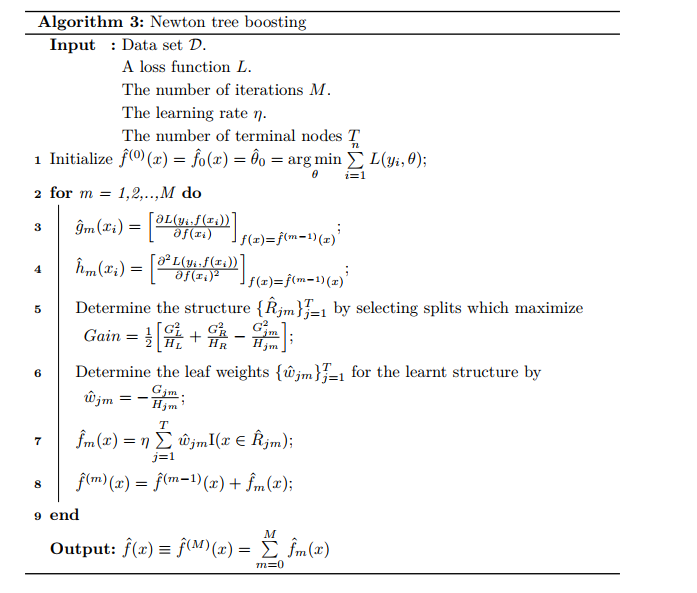
Note that,
\[G_{jm} = \sum\limits_{i \in I_{jm}} \hat{g}_m(x_i)\]and
\[H_{jm} = \sum\limits_{i \in I_{jm}} \hat{h}_m(x_i).\]Gradient Tree Boosting Algorithm
The gradient tree boosting algorithm is closely related to the gradient boosting algorithm shown in Algorithm 1. In line 4, a tree is learnt using the criterion
\[\tilde{J}_m (\phi_m) = \sum\limits_{i=1}^n \left[ (−\hat{g}_m(x_i)) − \beta \phi(x_i) \right]^2,\]which is an approximation to the FSAM criterion.

Comparison of Tree Boosting Algorithms
In this section, we will compare the two tree boosting algorithms discussed above. Recall that, at iteration $m$, both these two algorithms seek to minimize the FSAM criterion which can be rewritten
\[\{ \hat{w}_{jm}, \hat{R}_{jm} \}_{j=1}^{T_m} = \underset{ \{ w_{jm}, R_{jm} \} _{j=1}^{T_m} } {\arg\min} \sum\limits_{i=1}^n L(y_i, \hat{f}^{(m−1)}(x_i) + \sum\limits_{j=1}^{T_m} w_{jm} I(x_i \in R_{jm})).\]This is repeated for $m = 1, …, M$ to yield an approximation to the solution to empirical risk minimization problem.
Gradient tree boosting and Newton tree boosting however, differ in the tree structures they learn and how they learn the leaf weights to assign in the terminal nodes of the learnt tree structure.
Learning the Structure
Gradient tree boosting and Newton tree boosting optimize different criteria when learning the structure of the tree at each iteration.
-
Gradient tree boosting learns the tree which is most highly correlated with the negative gradient of the current empirical risk.
-
Newton tree boosting, on the other hand, learns the tree which best fits the second-order Taylor expansion of the loss function.
Learning the structure amounts to searching for splits which maximize the gain. For gradient tree boosting, this gain is given by
\[Gain = \frac{1}{2} \left[ \frac{G_L^2}{n_L} + \frac{G_R^2}{n_R} − \frac{G_{jm}^2}{n_{jm}} \right],\]while for Newton tree boosting, the gain is given by
\[Gain = \frac{1}{2} \left[ \frac{G_L^2}{H_L} + \frac{G_R^2}{H_R} − \frac{G_{jm}^2}{H_{jm}} \right].\]Newton tree boosting learns the tree structure using a higher-order approximation of the FSAM criterion. We would thus expect it to learn better tree structures than gradient tree boosting. The leaf weights learnt during the search for structure are given by
\[\tilde{w}_{jm} = − \frac{G_{jm}}{n_{jm}}\]for gradient tree boosting and by
\[\tilde{w}_{jm} = − \frac{G_{jm}}{H_{jm}}\]for Newton tree boosting. For gradient tree boosting these leaf weights are however subsequently readjusted.
Learning the Leaf Weights
After a tree structure is learnt, the leaf weights need to be determined. For Newton tree boosting, the final leaf weights are the same as the leaf weights learnt when searching for the tree structure, i.e.
\[\tilde{w}_{jm} = − \frac{G_{jm}}{H_{jm}}.\]Gradient tree boosting, on the other hand, uses a different criterion to learn the leaf weights. The final leaf weights are determined by separate line searches in each terminal node $j = 1, …, T$
\[\hat{w}_{jm} = \underset{w_j}{\arg\min} \sum\limits_{i \in \hat{I}_{jm}} L(y_i, \hat{f}^{(m−1)}(x_i) + w_j).\]Considering this, gradient tree boosting can be seen to generally use a more accurate criterion to learn the leaf weights than Newton tree boosting. These more accurate leaf weights are however determined for a less accurate tree structure.
Empirical Comparison
To get an idea of how they compare in practice, we will test their performance on two standard datasets, the Sonar and the Ionosphere datasets. The log-loss was used to measure prediction accuracy. We will use only tree stumps (trees with two terminal nodes) and no other form regularization of the individual trees.
The learning rate was set to $\eta = 0.1$ and the number of trees was set to $M = 10,000$. Predictions were made at each iteration. To get a fairly stable estimate of out-of-sample perfomance, three repetitions of 10-fold cross-validation was used. The folds were the same for both algorithms.
To study the effect of line search for gradient tree boosting, one fit were also done using gradient boosting with line search.


From figures above, we observe that NTB seems to outperform GTB slighly for the Sonar dataset. We can see that NTB converges slightly faster, but GTB outperforms NTB when run for enough iterations for the Ionosphere dataset. They do however seem to have very similar performance for both problems. Of course, due to randomness, any algorithm might perform best in practice for any particular data set.
We can also see that line search clearly improves the rate of convergence. In both cases, line search also seems to improve the lowest log-loss achieved. Line search thus seems to be very beneficial for gradient tree boosting.
Why Does XGBoost Win “Every” Competition?
We all know that, for any specific data set, any method may dominate others. In this section, we will thus provide arguments as to why tree boosting seems to be such a versatile and adaptive approach, yielding good results for a wide range of problems, and why XGBoost may outperform MART for many problem.
Generally, tree boosting is so effective because it fits additive tree models, which have rich representational ability, using adaptively determined neighbourhoods. The property of adaptive neighbourhoods makes it able to use variable degrees of flexibility in different regions of the input space. Consequently, it will be able to perform automatic feature selection and capture high-order interactions without breaking down. It can thus be seen to be robust to the curse of dimensionality.
For MART, the number of terminal nodes is kept fixed for all trees, which might be suboptimal. For example, for highdimensional data sets, there might be some group of features which have a high order of interaction with each other, while other features only have lower order interactions, perhaps only additive structure. We would thus like to use deeper trees for some features than for the others. If the number of terminal nodes is fixed, the tree might be forced to do further splitting when it is not necessary. The variance of the additive tree model might thus increase unnecessarily. In contrast, XGBoost uses clever penalization of the individual trees. The trees are consequently allowed to have varying number of terminal nodes.
Moreover, while MART uses only shrinkage to reduce the leaf weights, XGBoost can also shrink them using penalization. The benefit of this is that the leaf weights are not all shrunk by the same factor, but leaf weights estimated using less evidence in the data will be shrunk more heavily. Again, we see the bias-variance tradeoff being taken into account during model fitting. XGBoost can thus be seen to be even more adaptive to the data than MART.
In addition, XGBoost employs Newton boosting rather than gradient boosting. By doing this, XGBoost is likely to learn better tree structures.
Finally, XGBoost includes an extra randomization parameter. This can be used to decorrelate the individual trees even further, possibly resulting in reduced overall variance of the model.
References
Nielsen, D. (2016). Tree Boosting With XGBoost - Why Does XGBoost Win “Every” Machine Learning Competition?